Classification of Gene Expression Data through Distance Metric Learning:
Final
Mar 8th, 2013
Craig O. Mackenzie, Qian Yang
Introduction
One of the great promises of bioinformatics is that we may be able to predict health outcomes based on genetic makeup (and environmental factors). Classification of gene expression data is one way that this can be done. Gene expression levels are essentially measurements of how active genes are. The expression level for a gene is determined by the abundance of its messenger RNA (mRNA), the product of the gene that will be used as a template to make proteins. Proteins are the engines and building blocks of life and changes in the levels of proteins may indicate disease. There appears to be a correlation between mRNA and protein levels in certain studies, though this relationship is fairly complex. Even in cases where mRNA levels do not correlate with protein levels, they could still be an important factor in understanding disease.
The ultimate goal of gene expression classification is to predict whether someone has or will have a certain health outcome based on the expression levels of certain genes. These outcomes could be disease vs. control, stages of cancer, or subtypes of a disease. Depending on the classification method used, it may allow us to hone in on genes that discriminate the most between disease states, thus giving us biological insight into the disease. These problems also serve as great computational challenges to those working in the field of bioinformatics and machine learning. One must deal with the fact that there are usually thousands of genes and relatively few samples. A gene expression dataset can be thought of as a matrix where the rows represent patients (samples) and the columns represent genes (features).
Gene expression classification is a well-studied field and many computation methods have been used or developed for it. These include support vector machines, regression trees and k-nearest neighbors, to name a few. In our project we decided to use a modified k-nearest neighbor algorithm (kNN).
The k-nearest neighbor algorithm is one of the simplest
machine learning algorithms and classifies samples based on the closest
training samples in the feature space. The unlabeled sample is usually given
the class label that is most frequent among the k nearest training samples
(neighbors). This procedure of deciding the class label based on frequency is
referred to as “frequency” or “majority voting”. The kNN
algorithm has strong consistency in its results. As the data approaches
infinity, the error rate of the algorithm is guaranteed to be no more than
twice of that of Bayes
Methods
Modified kNN Classifier
We modified the classical kNN algorithm in two ways in order to test it on gene expression datasets.
The first modification was to the procedure used to assign class labels based on the k nearest neighbors. One of the drawbacks to the basic “frequency voting” (sometimes called “majority voting”) method is that the classes with more frequent examples tend to dominate the prediction of the new test sample. This could be a problem in gene expression classification, since the classes rarely have equal sizes. So we decided to also use minimum average-distance method in which a test sample is assigned the class with the closest centroid its k nearest neighbors. We also decided to modify the frequency voting method so that the classes were weighted by their relative sizes. This is simply accomplished by dividing the vote of each class, by the total number of samples in the class. There are more advanced methods of weighting votes (e.g. by the distance of each vote to the test sample), but we decided not to pursue this.
The second problem that we decided to tackle was that of selecting an appropriate distance metric. The kNN can be used with any distance metric appropriate for the data. In the case of real valued data, the Euclidean distance is a popular choice. However, in high dimension data, the Euclidean distance may not perform well. This is a great concern in gene expression data, where there are typically thousands of features (genes) present in the dataset. Other distance metrics could be chosen, but it is often hard to select an appropriate one that generally works well across datasets of a particular type. We decided to use distance metric learning to optimize performance in the kNN classifier. This method attempts to create a distance metric that make samples with the same class labels close to each other and those with different labels far apart.
In
Large Margin Component Analysis (LMCA)
We decided to use linear LMCA as it not only learns a Mahalanobis distance metric, but also reduces the dimensionality of the feature space. Instead of learning a distance metric, this method transforms the data so that using the Euclidean distance in the transformed space is equivalent to using the learned distance in the original space. Intuitively this space should be transformed so that samples with the same class labels are near to each other and those with different labels are further apart. Thus the goal of this algorithm is to find the matrix L that will transform the original space X in such a way. Note that L is a d × D matrix where D is the dimension of the data and d < D. Equation 1 gives the error function of the desired transformation.
![]()
(Equation 1)
Y is a matrix whose ijth
entry is 1 if samples i and j share the same class
labels. N is the matrix whose ijth entry
is 1 if sample j is a k-nearest neighbor of sample i
and it shares the same class label. c is a constant
and h is the hinge function. The first term in this equation encourages small
distances between samples sharing the same class labels and the second terms
encourages large distances between points sharing different labels. The hinge
function will be zero if ![]() is
less than or equal to
is
less than or equal to![]() .
This is a desirable result and thus we would want the repulsion term to be 0.
If
.
This is a desirable result and thus we would want the repulsion term to be 0.
If ![]() is
greater than
is
greater than![]() ,
then it will simply return this difference. Since there is no closed form
solution for minimizing
,
then it will simply return this difference. Since there is no closed form
solution for minimizing ![]() ,
we use a gradient descent method using equation to approximate this. Equation 2
gives the update rule for the gradient descent algorithm.
,
we use a gradient descent method using equation to approximate this. Equation 2
gives the update rule for the gradient descent algorithm.
![]()
(Equation 2)
The step size, α, is adjusted through the algorithm and the gradient is given in Equation 3.
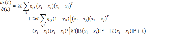
(Equation3)
Differentiation of the hinge function was handled by
adopting a smooth hinge function. We implemented gradient descent with line
search in our program. Another method we implemented was a simulated annealing
approach to the optimization of L in which we ran leave-one-out
cross-validation on the training data during the minimization of ![]() .
In this method we still updated L with equation 2. However, we would only except the “new” L if the error from kNN
on the transformed data had improved. We also accepted bad solutions with a
probability that decreased over time. This helps to avoid getting stuck in
local minimums. L can be initialized randomly or with PCA. In our program we
have these options along with the ability to slightly perturb the PCA
initialization.
.
In this method we still updated L with equation 2. However, we would only except the “new” L if the error from kNN
on the transformed data had improved. We also accepted bad solutions with a
probability that decreased over time. This helps to avoid getting stuck in
local minimums. L can be initialized randomly or with PCA. In our program we
have these options along with the ability to slightly perturb the PCA
initialization.
Finding the best choice of k is another challenging part of kNN algorithm. The optimum value of k depends on the dataset itself. Large values of k results in larger bias while smaller value of k contributes to a higher variance. We determined the best value or k in each dataset by testing a range of reasonable values for this hyper-parameter.
The LMCA algorithm also introduces two new hyper-parameters that we must attempt to optimize. The first is c, which is the weight given to the repulsion term and the second is d, the target dimension (number of rows in L).
Improving the speed of LMCA
Since the LMCA implementation was quite slow, we made some modifications to increase the speed.
In Equation 3, we could pre-compute ![]() and use it throughout gradient descent as it
did not rely on L. In the repulsion term we only summed over the terms where
the product
and use it throughout gradient descent as it
did not rely on L. In the repulsion term we only summed over the terms where
the product ![]() .
We serialized the outer products for those (i, j, k)
use the python shelve module.
.
We serialized the outer products for those (i, j, k)
use the python shelve module.
Datasets
The first dataset that we used is the colon cancer dataset
from
Another dataset that we used is the Scleroderma dataset from
Implementation
The classic kNN and modified LMCA were implemented in Python. We used (imported) the numpy, scipy and scikit-learn packages. Since the gene expression datasets are high dimensional, even after increasing the speed of LMCA, our program still ran fairly slow. We used a computing cluster to test out different parameter combinations. For the colon cancer dataset we tried reducing the dimension to 10, 20, 50, 100 and 200 with the LMCA algorithm. In the Scleroderma dataset we reduced the dimension 20, 50 and 100. For both datasets we tried values of c equal to 0.5, 1, 10, 100 and 1000. Due to time considerations we only used the frequency voting method and the minimum average distance method (although the weighted voting scheme is implemented in our program).
Evaluation Criteria
We calculated the
misclassification error rate to evaluate our predictions:
Error Rate = ![]()
Results
We compared distance
metric learning (LMCA), Euclidean and correlation distance using 5-fold cross
validation.
In our experiments,
there did not appear to be much difference across the various choices of the
reduced dimension or values of c. For the Colon Tumor dataset, we chose to
present the results with reduced dimension with LMCA to 50. This reduced
dimension seemed to perform slightly better than the others when averaged out
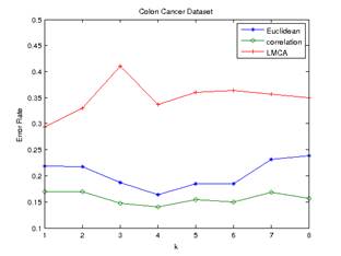
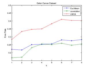
over values of k. The error rates of predictions generated by frequency voting
and minimum average distance are shown in Figure 1 and Figure 2 below.
Figure 2.Error
Rate of Minimum Average Distance (colon cancer) Figure 1.Error
Rate of Frequency Voting (colon cancer)
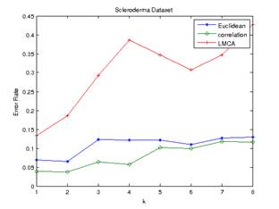
For the Scleroderma
dataset, the best reduction obtained using LMCA was 100. The error rates of
predictions generated by frequency voting and minimum average distance are
shown in Figure 3 and Figure 4 below.
Figure 4.Error Rate of Minimum
Average Distance (scleroderma dataset) Figure 3.Error Rate of Frequency
Voting (scleroderma dataset)
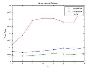
To our surprise, the
Euclidean and Pearson-correlation distances outperformed distance metric
learning in both datasets. The Pearson correlation distance seemed to perform
best in all cases. Even though the datasets are high dimensional with small
numbers of samples, Pearson correlation distance seems to have a relatively low
and stable error rate.
In the colon cancer
dataset, LMCA has the lowest error rate at k=1 (optimum value of k at 1) for
both frequency voting and minimum average distance method. Euclidean distance
has an optimum value of k at 4 for frequency voting method, and an optimum
value of k at 2 for minimum average distance method. Pearson-correlation
distance has an optimum value of k at 4 for frequency voting method, and
optimum value of k at 1 for minimum average distance method.
In the scleroderma
dataset, the minimum average distance method appeared to perform better than the
majority voting scheme in this dataset. LMCA still have the optimum value of k
at 1 for both frequency voting and minimum average distance method. Both
Euclidean and correlation distance have the optimum value of k at 2 for both
the frequency voting and minimum average distance method.
Discussion
There are many reasons
that may have caused the poor performance in the LMCA method in our experiments.
First the datasets contained a small number of samples while having a large
number of features. This is general not an ideal situation for a machine
learning problem. To make matters worse, we did 5-fold cross validation instead
of leave-one-out cross validation. We chose 5-fold cross validation due to the
computationally intensive nature of this algorithm. Using leave-one-out
cross-validation on the Scleroderma dataset would have taken 15 times as long
as 5 fold cross validation. Depending on the settings of different parameters,
the running time of 5 fold cross validation ranges from the 5 minutes to 12
hours.
While we tried
numerous choices for the hyper-parameters c and d, we were again limited by
computational resources in exploring a more values. Thus we may have missed the
ideal parameters for the algorithm. While we tried two different gradient
descent methods, there did not seem to be a clear performance difference (in
terms of error rate). Maybe another gradient descent or optimization method would have been better.
Again since the program took so long to run, it was somewhat difficult to
evaluate many different training options.
Lastly, the package we
were using to perform PCA initialization of L would not work on the computing
clusters. Due to other problems we had getting the program to run correctly on
the cluster, we were not able to figure out a way to use this or any other similar
package on the cluster machines. Even after doing a few small runs on our
personal computers with PCA initialization we did not see much improvement in
error rates. It should be noted that when running on our personal computers we
had to reduce the number of iterations for gradient descent and could not many
explore hyper-parameters choices.
Future Work
In the future, we would
like to test LMCA on datasets with more samples, which might be a better fit
for this machine learning algorithm. In addition, successfully performing PCA
to initialize L on the computing cluster would be a promising approach to
achieve better performance for LMCA. We would also like to try different
gradient descent approaches to see if we could better minimize the error
function for L. To really make this algorithm usable in our research will have
to write it in a lower level programming language such as C++ or Java and maybe
parallelize parts of it. This would allow for better testing of parameters and
training options.
Works Cited
Alon, U., Barkai, N., Notterman, D. A., Gish, K.,
Ybarra, S., Mack, D., et al. (1999). Broad Patterns of Gene Expression
Revealed by Clustering Analysis of Tumor and Normal Colon Tissues Probed by
Oligonucleotide Arrays. Proceedings of the National Academy of Sciences of
the United States of America, 6745-6750.
Bremner, D., Demaine, E., Erickson, J., Iacono, J.,
Langerman, S., Morin, P., et al. (2005). Output-sensitive algorithms for
computing nearest-neighbor decision boundaries.
Cover, T., & Hart, P. (1967). Nearest neighbor
pattern classification. IEEE Transactions on Information Theory, 21-27.
Sargent, J., Milano, A., Connolly, M., &
Whitfield, M. (n.d.). Scleroderma gene expression and pathway signatures.
Torresani, L., & Lee, K.-c. (2006). Large Margin
Component Analysis.
Weinberger, K. Q., Blitzer, J., & Saul, L. K.
(2006). Distance Metric Learning for Large Margin.
Xiong, H., & Chen, X.-w. (2006). Kernel-based
distance metric learning for microarray data. BMC Bioinformatics.